Problem Definition

The main challenge with predicting future cryptocurrency prices is the constant fluctuations and volatility of the market. Our original plan was to target important stats, such as market capitalization, volume or transactions, and daily closing prices. Using these stats, we organized them based on weeks instead of days. When shown visually, dividing the data by week instead of day allows for better visualizations. Using a long short-term memory (LSTM) model and an autoregressive integrated moving average (ARIMA), the algorithm can be trained on data from earlier years and use this to predict future data, or in our case cryptocurrency prices.

Data Collection

Bitcoin historical data was taken from Yahoo finance. The closing price after each day was the feature in question, and the following 5 features were used to predict the closing price: the open price, high price, low price, transaction volume, and market capitalization. Any missing data was filled by using forward fill, which propagates the last valid observation forward.

MODEL 1: Long Short-Term Memory

Methods

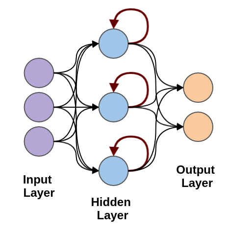
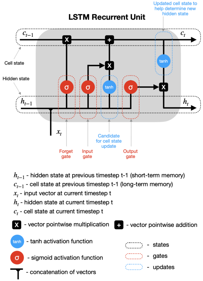
A LSTM (long short-term memory) Neural Network differs from a standard Feed-Forward Neural Network in that it can process sequential data. LSTM contains hidden layers with recurrence units at each node. The recurrence unit combines the input from the previous layer with a hidden state and a cell state from the previous timestep, which hold the short-term and long-term memory of the data respectively. In addition, there are also various gates in the unit that filters the data that is kept in these states.

Results and Discussion

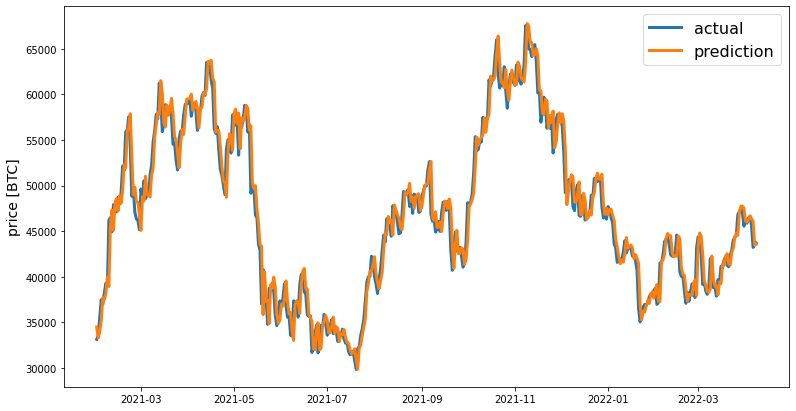
The results we obtained through our LSTM Neural Network model are depicted below. These results compare the closing prices predicted by our LSTM Neural Network model and the actual closing prices based on the training dataset. As shown in the graph, our LSTM Neural Network model offers decent prediction accuracy with very minimal errors/losses.

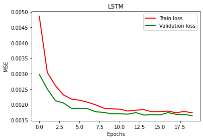
The mean squared error losses for the training dataset and the validation dataset were also calculated after every epoch, as shown below. It is observed that the losses seem to decrease minimally and even plateau after the 10th or 11th epoch.

To evaluate the performance of our LSTM Neural Network model, we calculated the mean absolute error, mean squared error, and the R2 score metrics. After running a total of 20 epochs to train our model, we obtained a mean absolute error of 0.02962258532033467, mean squared error of 0.0016351940958689334, and an R2 Score of 0.7780970097665939. As a rule of thumb, it is considered that RMSE values between 0.2 and 0.5 show that the model can relatively predict the data accurately, and that R2 score of more than 0.75 is a very good value for showing the accuracy.

MODEL 2: Autoregressive Integrated Moving Average

Methods

Automatic Time Series Decomposition is an essential part before running the model and obtaining loss values was to check the characteristics of the time series data using the statsmodels module. Decomposition is used as an analysis tool for time series data because it can be used to inform forecasting models. The seasonal_decompose function in statsmodels library allowed us to decompose the series into trend, seasonal, and residual components. The results are obtained by first estimating the trend by applying a convolution filter to the data. The trend is then removed from the series and the average of this detrended series for each period is the returned seasonal component. To obtain better visualizations of the decompositions the data was grouped week-wise before plotting the graphs again. The data was then further grouped into months to return better predictions.

Time series have several characteristics like trend (mean varying over time), seasonality ( time frame variations) etc. Time series are considered stationary if they don't have any trends or seasonal effects and properties like mean, autocorrelation, etc. are constant over time. When a time series is made stationary, it also becomes easier to model. The Augmented Dickey-Fuller test allows us to analyze the stationary of our data. From the p-values obtained on performing the test, we can make an inference as to whether a given time series is stationary or not. If the p-value returned by the ADF test is lesser than 0.05, then the data can be considered stationary. Since the initial p-value is 0.969, further steps must be taken to make the data stationary.

Differencing is a transformation that helps stabilize the mean of the time series which eliminates trend and seasonality. Since the data is grouped by month, there are 12 periods in a season. So, for seasonal differencing, we have taken the difference between each observation and the observation from 12 periods before. Since a trend is present in the data we also needed to perform non-seasonal differencing. At the end of this process, the Augmented Dickey-Fuller test is performed again and the p-value is observed to be 0.005.

The predictions are done using the Autoregressive Integrated Moving Average (ARIMA) method, which is capable of generating high accuracy in short-term predictions. There are three parameters p,d,q that account for:

p - the number of lag observations

d - the number of times that the raw observations are differenced

q - the size of the moving average window

We used a grid search approach to construct different parameter combinations so that the optimal set of parameters can be found to obtain the best performance for the ARIMA model. We then fitted the model and plotted the real and predicted prices.

Results and Discussion

An essential part before running the model and obtaining loss values was to graph out seasonality graphs. To get a better understanding of our possible predictions, the statsmodel library was used to find the Observed, Trend, Seasonal and Residual graphs for our dataset. Though the data correlated to actual trends as observed in real life from 2016 to 2022, the seasonal graph was very closely compressed since our dataset was too large as it grouped daily price updates.

To solve this problem, price updates were grouped on a week-to-week basis to accommodate for seasonal trends. On reviewing this graph, we were very satisfied with how we could trace back the observed trends to actual happenings.

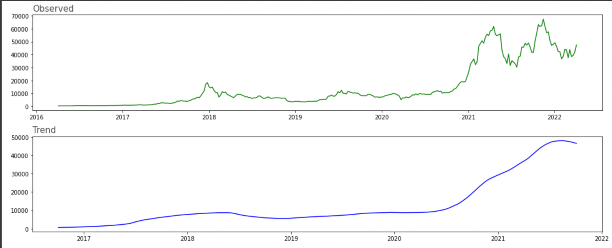
For example, the “Trend” graph supports the flattish nature of crypto in 2016 and 2017 before it began to start getting popular with crypto enthusiasts in 2018. Crypto prices then took a slight hit in 2019 when Bitcoin and Ethereum went through a “winter phase” and have since risen as cryptocurrencies and tokens have become mainstream. Modeling our dataset to correlate our findings to actual price changes was a task.

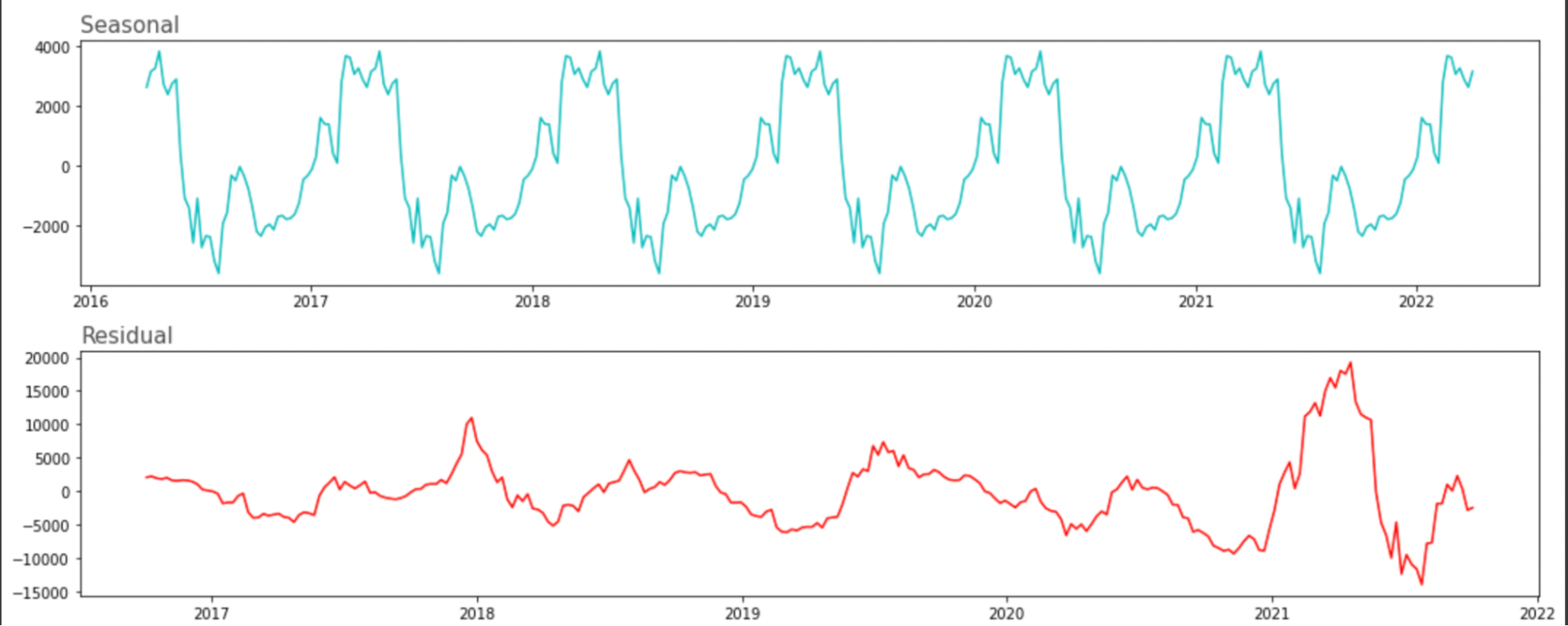
Other trends that can be seen are that there is a seasonal variation to crypto prices from about 4000 to -2000 and that most of the noise was generated in the 2018 - 2019 crypto-hype phase.

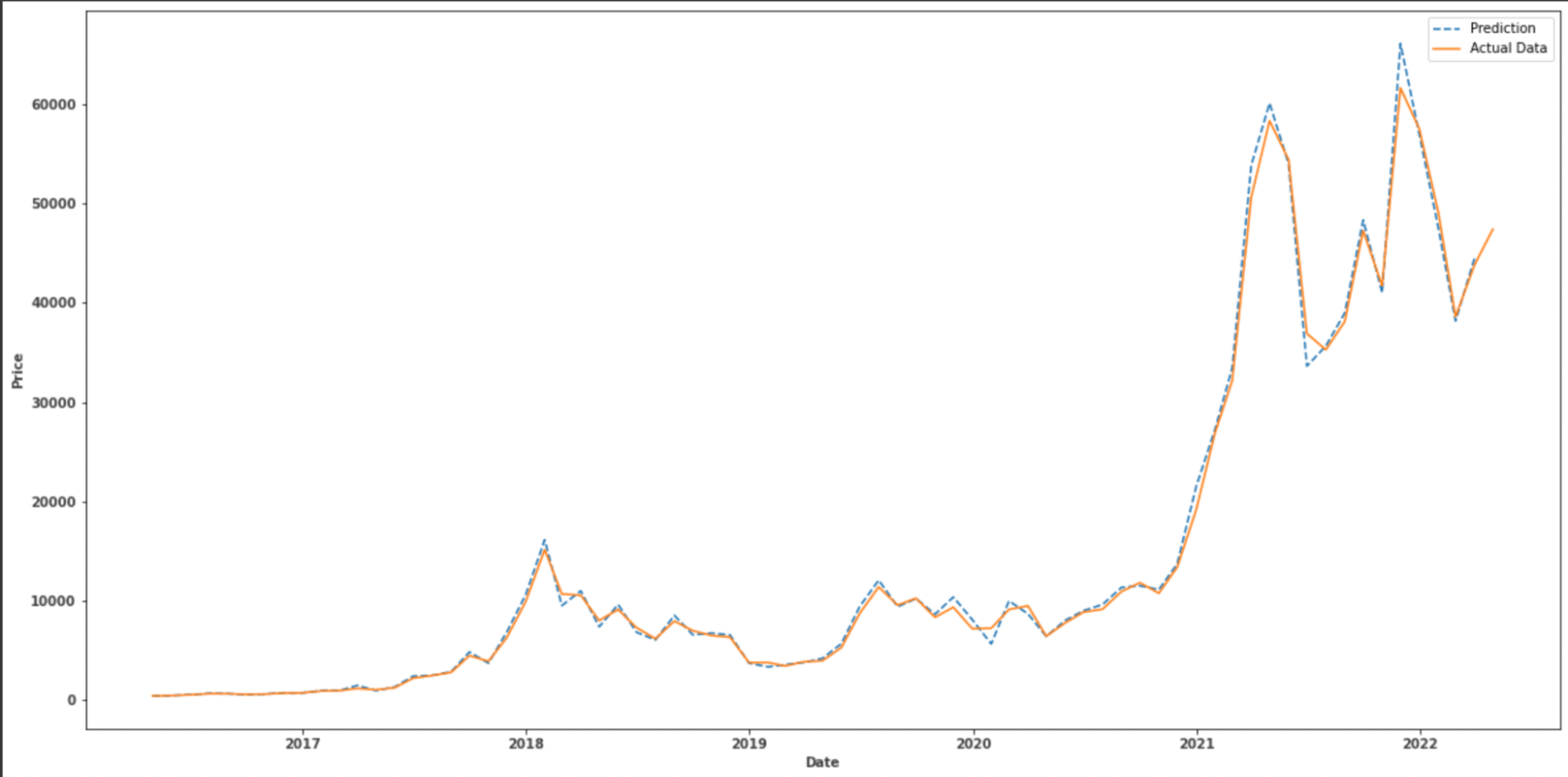
ARIMA, short for ‘Auto Regressive Integrated Moving Average’ is actually a class of models that ‘explains’ a given time series based on its own past values, that is, its own lags and the lagged forecast errors, so that equation can be used to forecast future values. We chose the ARIMA algorithm to model the data because ARIMA can use stationary values well to fit short term data.

The graph below shows how closely the predicted prices mirror the actual prices. This model offers a good prediction accuracy and to be relatively fast compared to other alternatives, in terms of training/fitting time and complexity.

Works Cited

[1] Aharon, D. & Qadan, M., 2022. Bitcoin and the day-of-the-week effect. Science Direct. https://doi.org/10.1016/j.frl.2018.12.004.

[2] Sebastião, H., & Godinho, P. (2021, January 6). Forecasting and trading cryptocurrencies with machine learning under changing market conditions - financial innovation. Financ Innov 7, 3 (2021). https://doi.org/10.1186/s40854-020-00217-x.

[3] Weinhardt, Patrick Jaquart and David Dann and Christof. Short-term bitcoin market prediction via machine learning. https://doi.org/10.1016/j.jfds.2021.03.001.

[4] Levy, A. (2021, October 6). What makes cryptocurrency go up or down? The Motley Fool. Retrieved April 8, 2022, from https://www.fool.com/investing/stock-market/market-sectors/financials/cryptocurrency-stocks/value-of-crypto/

[5] Cryptocurrency market. Market Research Firm. (n.d.). Retrieved April 8, 2022, from https://www.marketsandmarkets.com/Market-Reports/cryptocurrency-market-158061641.html